A tale of two kernels
For developers integrating Haskell into data science workflows or interactive documentation, the Jupyter notebook is the standard interface. Currently, there are two primary ways to run Haskell in Jupyter: IHaskell and xeus-haskell.
While both achieve the same end user experience (executing Haskell code in cells) their internal architectures represent fundamentally different engineering trade-offs:
- IHaskell: “Do everything in Haskell.” It is a monolithic kernel that speaks the Jupyter protocol itself and drives GHC directly.
- xeus-haskell: “Reuse the protocol machinery.” It delegates all protocol handling to a shared C++ framework (Xeus) and focuses only on connecting that framework to a Haskell interpreter (MicroHs).
This article explores those architectures side-by-side, with a focus on:
- How they plug into the Jupyter kernel model.
- What their design implies for performance, deployment, and library compatibility.
- Which one is likely the better fit for different use cases (data science, teaching, documentation, client-side execution, etc.).
The Jupyter Kernel Architecture
Jupyter is essentially a front-end that communicates with a computation server via a protocol (aptly called the Jupyter protocol). This computation server is called a kernel. All jupyter needs to know about a kernel is which ports to use to communicate different kinds of messages.
To understand the difference between IHaskell and xeus-haskell, we must first look at the “Kernel” abstraction. Jupyter is essentially a decoupled frontend (the web UI) that communicates with a computation engine (the Kernel) via a standardized protocol over ZeroMQ (ØMQ).
The Jupyter stack looks like this:
- JupyterLab / Notebook frontend (browser): Renders notebooks, lets you edit cells, handles user events.
- Jupyter server (Python): Manages files, launches kernels, proxies messages.
- Kernel (language backend): Actually executes your code.
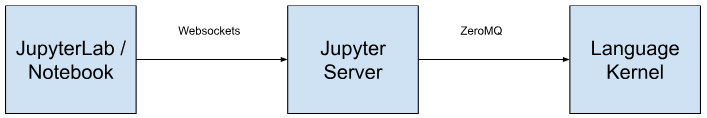
The frontend and the kernel do not share memory. They talk over five distinct logical channels, each responsible for a specific type of message exchange:
- Shell: The main request/reply loop. The frontend sends code execution requests here.
- IOPub: A broadcast channel. The kernel publishes “side effects” here, such as stdout, stderr, and renderable data (plots, HTML).
- Stdin: Allows the kernel to request input from the user (e.g., when a script asks for a password).
- Control: A high-priority channel for system commands (like “Shutdown” or “Interrupt”) that must bypass the execution queue.
- Heartbeat: A simple ping/pong socket to ensure the kernel is still alive.
From Jupyter’s perspective, a “Haskell kernel” is just a process that:
1) Reads a connection file to discover what ports to bind to. 2) Speaks the protocol correctly on those five channels. 3) Evaluates Haskell code when asked, and sends back results.
Everything else is an internal design choice.
The Registration Spec
Jupyter discovers kernels via a JSON specification file (kernel.json). You can list these with jupyter kernelspec list. A typical spec looks like this:
{"argv":["/home/yavinda/.cabal/bin/ihaskell","kernel","{connection_file}","--ghclib","/usr/lib/ghc/lib","+RTS","-M3g","-N2","-RTS"],"display_name":"Haskell","language":"haskell"}
When Jupyter starts a kernel, it generates a connection file (represented by {connection_file} in the args above). This ephemeral JSON file tells the kernel which ports to bind to for the five channels:
{
  "shell_port": 41083,
  "iopub_port": 42347,
  "stdin_port": 56773,
  "control_port": 57347,
  "hb_port": 34681,
  "ip": "127.0.0.1",
  "key": "aa072f60-5cac0ac2506b1a572678209a",
  "transport": "tcp",
  "signature_scheme": "hmac-sha256",
  "kernel_name": "haskell"
}
Some notable fields:
- Ports: One per channel (shell_port, iopub_port, etc.).
- Key + signature_scheme: Used to sign messages (HMAC) so rogue processes can’t spoof messages.
- Transport + IP: Usually TCP over localhost, but in principle could be remote.
Each of these ports is used to send different types of payloads to the kernel. So any implementation of the Jupyter protocol needs to handle these messages correctly (or at least, gracefully).
Both IHaskell and xeus-haskell parse this file and bind to these ports. The difference lies in how they implement the logic behind these sockets. IHaskell takes full responsibility for the protocol and evaluation. xeus-haskell lets Xeus (C++) handle protocol details and just plugs in a Haskell interpreter.
IHaskell’s architecture - the monolithic approach
IHaskell is a native Haskell implementation of the Jupyter protocol. It is a standalone binary that links against the GHC API and the ZeroMQ C bindings.
How it works
When you run IHaskell, you are running a Haskell executable that manages the entire lifecycle:
- Protocol Layer: IHaskell uses Haskell libraries (like zeromq-haskell) to listen on the sockets directly. It manually serializes and deserializes the JSON messages defined by the Jupyter protocol.
- Execution Layer: It uses the GHC API to act as an interactive execution environment. It effectively functions as a custom GHCi (REPL) instance wrapped in a network server.
Because IHaskell is the protocol implementation, it has to know and implement all of Jupyter’s message types and semantics itself. That’s a lot of fairly dull plumbing, but the payoff is a kernel that’s deeply integrated with GHC.
Architecture Nuances
Because IHaskell is a “thick” wrapper around GHC, it supports the full weight of the GHC ecosystem. Any library compatible with your system’s GHC can be loaded. However, this tight coupling means IHaskell is sensitive to GHC versions. If you upgrade your system compiler, you must often recompile IHaskell to match. IT’s no suprise then that most complaints around IHaskell are around installation and package management. You inherit all the complexity of GHC and your package manager while simultaneously trying to communicate with a client.
Xeus-haskell: The Middleware Approach
Xeus takes almost the opposite view: separate the Jupyter protocol from the language implementation.
Xeus is a C++ library implementation of the Jupyter protocol. It abstracts away the complexity of managing ZeroMQ sockets, message signing, and concurrency. Xeus-haskell is not a standalone implementation of the protocol. rather, it is a binding between the Xeus C++ library and a Haskell interpreter.
In this architecture, the “Language Kernel” box is split in two:
- The Frontend (C++): Xeus handles the connection file, the heartbeat, and message validation. It implements the “boring” parts of the Jupyter spec.
- The Backend (Haskell): The kernel implementer only needs to subclass a few C++ virtual methods.
MicroHs
Xeus-haskell uses MicroHs as its engine. MicroHs is a small Haskell implementation, designed to be compact and simple. It implements a substantial subset of Haskell (roughly Haskell 2010 with some additions), but not the entire surface area of modern GHC.
This has some very tanglible benefits. Firstly, it has a much smaller runtime footprint so it’s easier to port to environments like WebAssembly (WASM). Secondly, (mostly related to the first point) it has a faster cold-start and simpler distribution.
The tradeoff, however, is that you can’t just cabal install any random GHC package and expect it to work. Advanced GHC features (Template Haskell, fancy type-level programming, certain extensions) may be unsupported or behave slightly differently.
Maintainance
Xeus’ architecture allows kernel writers to focus more on writing the kernel and less on ceremonious communication with the Jupyter client. A kernel author doesn’t need to reinvent message dispatch, heartbeat and control channels, content-type negotiation, rich display MIME handling etc. Instead, you implement a handful of methods like “execute this code” and “generate completions,” and Xeus wraps that in a fully compliant kernel.
Also, because the protocol logic is offloaded to the shared Xeus C++ library, updates are “free.” If Jupyter releases a new feature (like Debugger Protocol support), Xeus updates it for all supported languages (C++, Python, Lua, Haskell) simultaneously. Whereas IHaskell would have to write all the plumbing that supports the feature.
Differences
How they are run
Because the protocol implementation (Xeus) and the interpreter (MicroHs) are relatively small, xeus-haskell can be compiled to WebAssembly and run entirely in the browser (e.g. with JupyterLite or other WASM-hosted frontends). This enables client-side Haskell notebooks since there are no server kernel processes and there is no separate toolchain on the user’s machine.
IHaskell, by contrast, is built around the full GHC toolchain and runs either directly on your machine or in a containerized environment like Docker. This gives IHaskell a higher baseline of power and compatibility, but makes it much less suitable for pure client-side environments.
Ecosystem
Xeus only works with MicroHs compatible libraries (currently few but growing in number) whereas IHaskell works with any library in the GHC ecosystem.
Ease of use
Installation experience is where xeus-haskell tends to shine.
IHaskell needs a matching GHC version and often a specific build tool to smooth over dependency issues. The kernel itself (and the packages it uses) needs to be built with the same GHC that your notebooks will use. This is absolutely doable (and there are Docker images/VS Code devcontainers that make it trivial), but if you try to install IHaskell “natively” on a system with multiple GHCs and mixed tooling, it can be … educational.
xeus-haskell comes as a relatively self-contained package. You’re not wrangling the entire GHC ecosystem; you’re picking up MicroHs plus the kernel parts. The time between download to first-notebook-command in Xeus-Haskell could be as little as 5 minutes.
Execution model and performance
Both kernels are fundamentally interactive REPLs with state that accumulates over cells. Althought GHC code typically runs about 10 time faster than MicroHs code, in a xeus notebook the entirety of MicroHs is interpreted. This increases the performance gap.
In practice, for “toy” examples and teaching, both are fast enough. For heavier workloads (e.g. large dataframes, numeric computing, deep learning), IHaskell’s access to the full GHC ecosystem and native performance is a big advantage.
You can try both yourself to see the difference:
Deployment scenarios
Different architectures lend themselves to different deployment stories.
IHaskell is great for server-side notebooks. You can containerize IHaskell and ship it with JupyterHub on a cluster where each user gets an IHaskell kernel. Or you can use services like mybinder which work with Docker containers that already have Jupyter bundled.
Where does this leave Xeus-haskell? Xeus-Haskell us great for quick prototyping or for places where you’d like to embed Haskell without inheriting the whole toolchain. Think demos, talks, small/static websites.
In the words of the project’s creator (@tani):
The goal is to make Haskell more accessible in scientific/technical computing. Lazy evaluation can be surprisingly powerful for graph algorithms, recursive structures, and anything where “compute only what’s needed” brings real wins. Being able to demo that interactively in a notebook feels like the right direction.
Conclusion
For standard server-side data science, IHaskell remains the battle-tested standard. However, if you are building lightweight interactive documentation or require client-side execution (JupyterLite), xeus-haskell offers a compelling, modular architecture.
Both solutions have found usecases in DataHaskell and we’re excited to keep iterating on them to improve the Haskell data ecosystem.